These are a few papers I found interesting either by the work itself or the concepts/techniques it used, although the concept/techniques might be old.

Paper 1: Inpainting with Diffusion Model

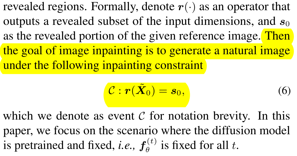
Problem Setting

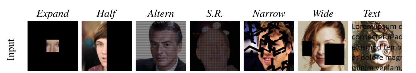
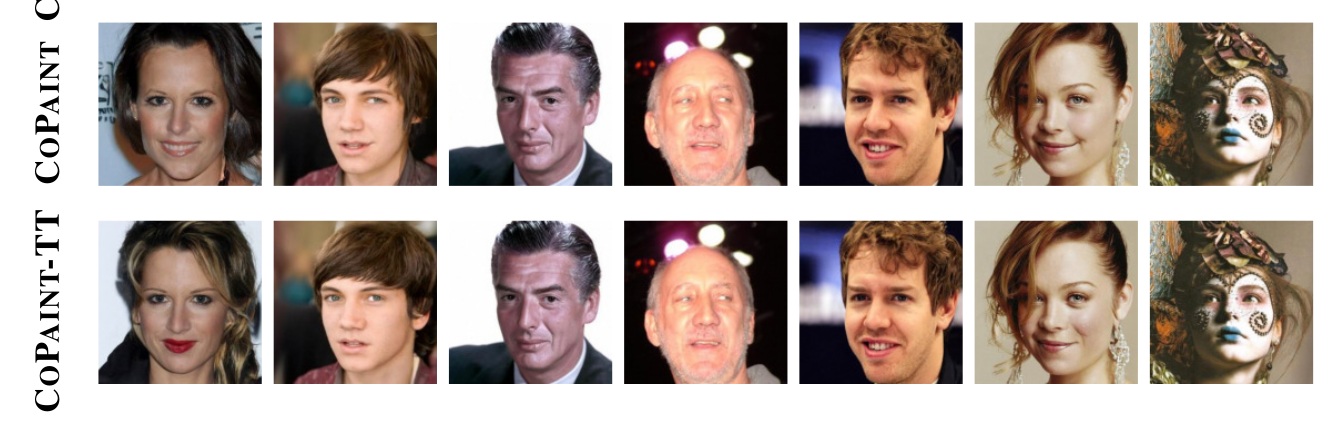
Given a partially masked image where the shape of the mask is arbitrary, generate the hidden part to produce a complete image. Here is a demonstrate from the paper (part of Figure 9), where the black areas represent the missing part of the input images.

Review on Diffusion

Forward diffusion dynamic:

where ( x^2=6 ), $\textbf{x} \in \mathbb{R}^{d}, \textbf{w} \in \mathbb{R}^{d}$ and $\textbf{f}(\cdot,x):\mathbb{R}^{d} \to \mathbb{R}^{d}, \textbf{G}(\textbf{x}, t): \mathbb{R}^{d} \to \mathbb{R}^{d \times d}$.

Note that functions $\textbf{f}, \textbf{G}$ are pre-specified and fixed.

(Anderson, 1982) shown that we can model the dynamic if time travels in the backward direction as

Now if $\textbf{x}$ is generated conditioning on some $\textbf{y}$, the same recipe is still applicable. In particular, we can think of describing a collection of diffusion processes (instead of a single diffusion process) indexed by $\textbf{y}$.
The forward of these diffusion processes would be exactly identical to each others as the forward describes how to diffuse the input $\textbf{x}_0 = \textbf{x}$ and knowing $\textbf{y}$ does not affect those processes. In contrast, the backward of these diffusions are different, i.e., \(\begin{equation} d\textbf{x} = \Big(\textbf{f}(\textbf{x}, t) - \nabla \cdot [\textbf{G}(\textbf{x}, t) \textbf{G}(\textbf{x}, t)^{\sf T}] - \textbf{G}(\textbf{x}, t)\textbf{G}(\textbf{x}, t)^{\sf T} \nabla_{\textbf{x}} {\color{green} \log p_t(\textbf{x} \mid \textbf{y}})\Big) dt + \textbf{G}(\textbf{x}, t) d \overline{\textbf{w}}. \end{equation}\)

This is also the reasoning behind classifier guidance diffusion method, as \(\log p_t(\textbf{x} \mid \textbf{y}) = \log p_t(\textbf{y} \mid \textbf{x}) + \log p_{t}(\textbf{x}).\)

In any case, if we have access to $\log p_t(\textbf{y} \mid \textbf{x})$, then we can use an unconditional generative diffusion model to generate samples conditioning on $\textbf{y}$.

Possible solutions:

We can always train a conditional generative model with the pair of (partially masked image, full image). But this might not be well generalizable since the mask shape is arbitrary. Instead, training an unconditional generative model is much easier since the unlabeled image data are abundant.

One solution for inpainting with diffusion model was written in the appendix of (Song, 2021). Denote $\textbf{x} = (\Omega(\textbf{x}), \Omega^{c}(\textbf{x}))$ corresponds to the revealed and missing part of the input image $\textbf{x}$. Then the inpainting problem can be cast to the conditional generative framework is: How to generate $\Omega^{c}(\textbf{x})$ given $\Omega(\textbf{x})$? Specifically, how to estimate ${\color{green}\log p_{t} (\Omega^{c}(\textbf{x}) \mid \Omega(\textbf{x}_0))}?.$

(Song, 2021) suggests an approximation like this

where the last approximation can be understood as we estimate the expectation by evaluating the function at a randomly drawn sample $\widehat{\Omega}(\textbf{x}) \sim p_t(\Omega(\textbf{x}) \mid \Omega(\textbf{x}_0))$. This sample drawing is pretty easily as it is defined by the forward process, and we can increase its precision by draw more than one sample. The first approximation, however, I haven’t figured out how it worked as well as how accurate it was. But my hunch is that it isn’t very good, otherwise people will just stop working on inpainting problem which is not the case.

Another suggestion which looks a bit heuristic to me was proposed in (Song, 2020), also in the appendix.

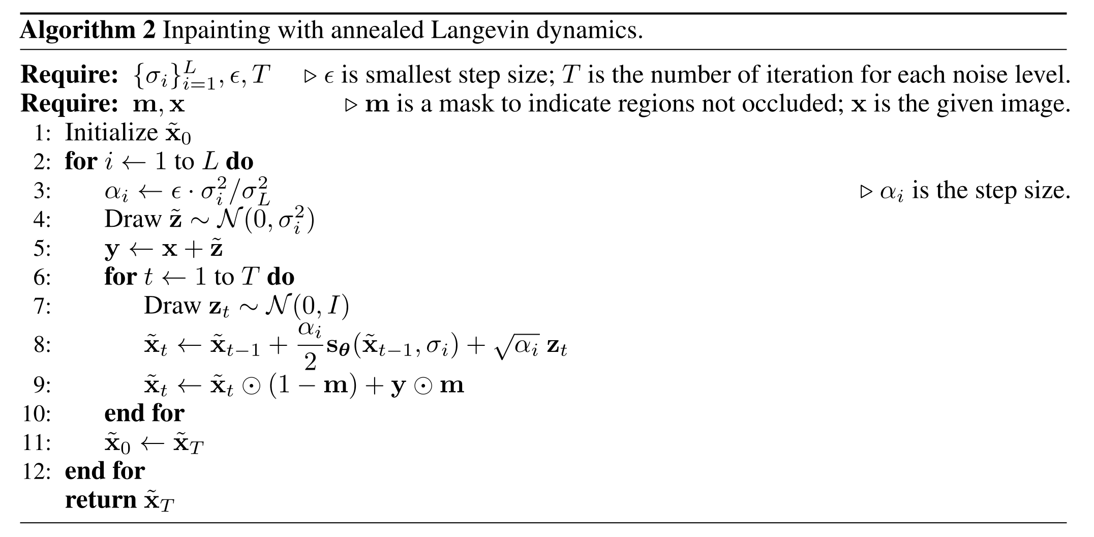
Not sure if these 2 approaches are related. But again, inpainting demonstration was not the main focus in this work either.

Now to the “real work”. 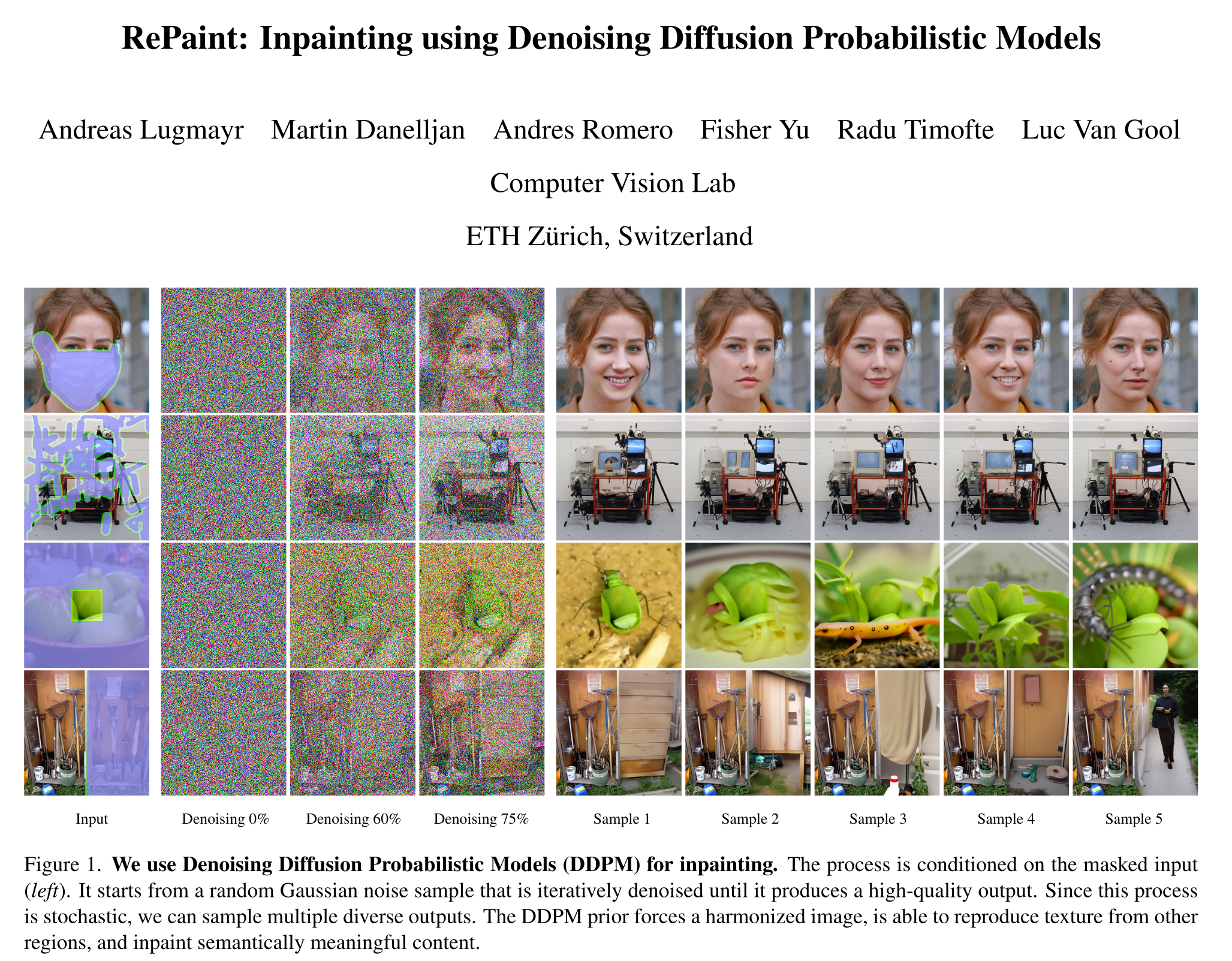I had a hard time trying find the novelty of this work in comparison to (Song, 2020). Here is all I found from the paper

In any case, here is the brief overview of their solution:

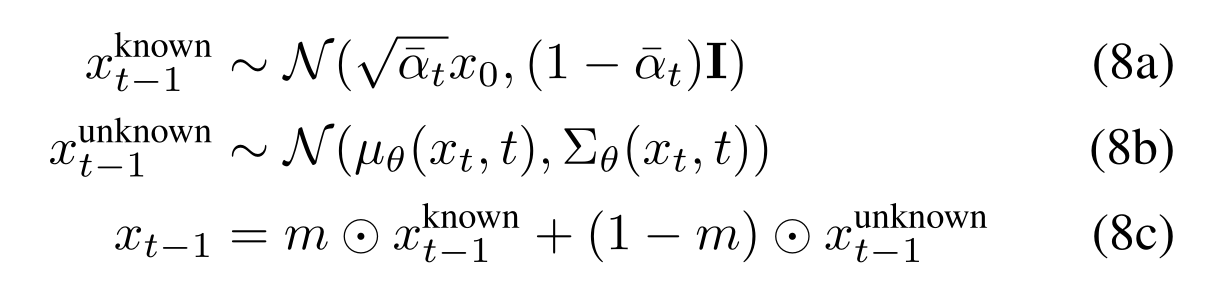
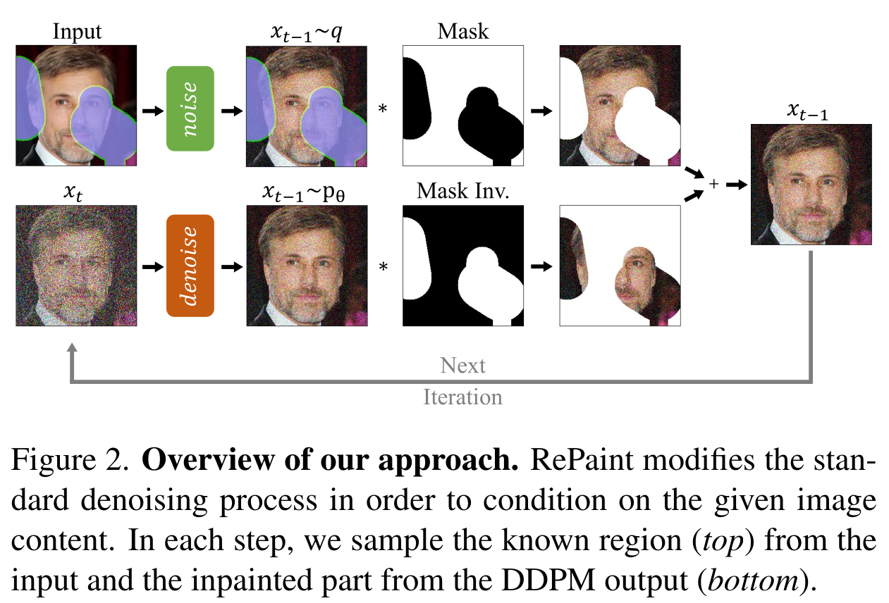
Originally, only with that solution, they got ‘ehhh’ quality-wise samples, and so they proposed another technical idea called resamples to improve the coherence of generated images:

That leads to our target paper published in ICML 2023.

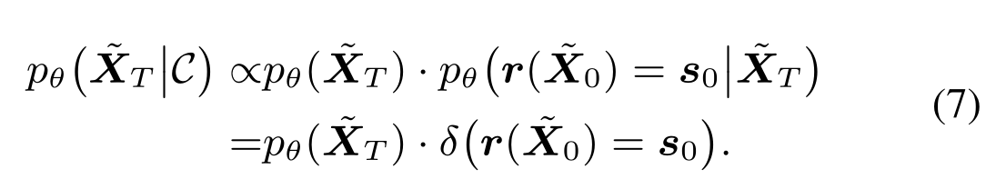
Previous limitations

The issue with previous approaches is that:

Their solution

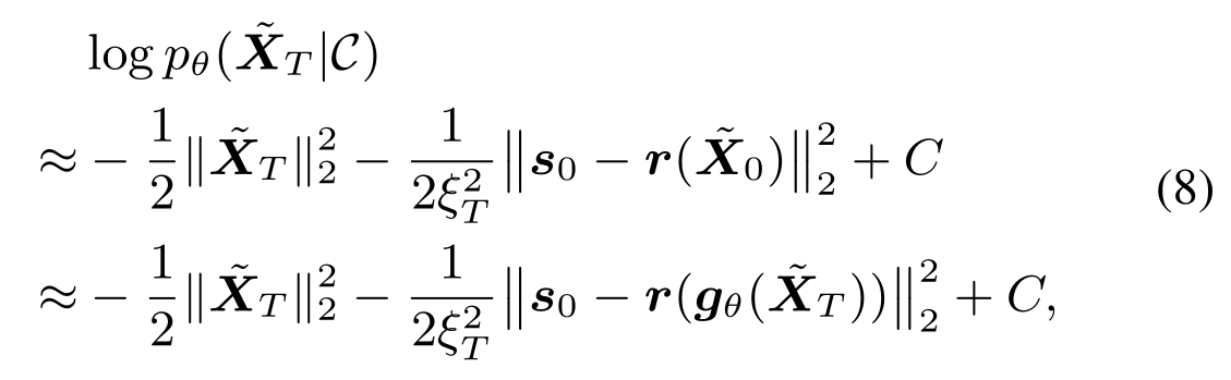
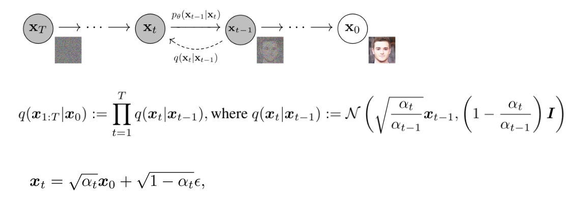
The simple version of their solution consider $\textbf{g}_{\boldsymbol \theta}(\cdot)$ that maps $\widetilde{\textbf{X}}_T$ to $\widetilde{\textbf{X}}_0$ is a deterministic mapping, which can be realized pratically with DDIM diffusion model. Under this view, what they are doing is essentially the same as optimizing over the latent vector to satisfy certain constraint, same as in GAN. And then of course, they will have to exploit/take into account properties of diffusion somewhere in the pipeline.

Indeed, the gradient over $\textbf{g}_{\boldsymbol \theta}(\cdot)$ would be super costly. So they proposed to use “one-step approximation”.

where $\textbf{f} _{\boldsymbol \theta}^{T}(\textbf{x}) \approx \textbf{g} _{\boldsymbol \theta}(\textbf{x})$.

But different from \(\textbf{g}\) where it requires to undergo 10-100 iterations, \(\textbf{f}_{\boldsymbol \theta}\) has a closed-form expression. The function \(\textbf{f} _{\boldsymbol \theta}\) is defined based on the following relation

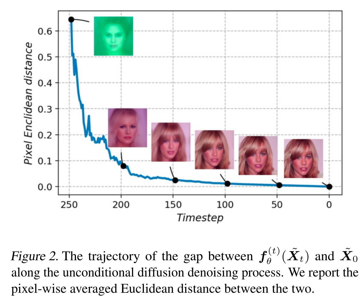
And they do have certain empirical evidence that the $\textbf{f}_{\boldsymbol \theta}$ should be an okay estimate of $\textbf{g}$,

Then they move to the general case where the backward process is stochastic. In this case, they will try to perform the same optimization at very iteration of the backward process. In principle, it is not the optimal way to do inference. To see that,

Note that only $\widetilde{\textbf{X}} _T$ is the variable in previous case, but in this case all $\widetilde{\textbf{X}} _{t}, t=0..T$ are variables. So their practical strategy is to use greedy approach, i.e., only optimize over $\widetilde{\textbf{X}}_t$ at iteration $t$.

My main concern about this method is running time, since the optimization is over image space which could be large, and also it is needed for every steps in the backward process. In their exp, they only run 1 step of gradience ascent, and show that it is faster than the state-of-the-art while having comparable quality (quite surprising). Refer to Figure 3 in the paper.

On the same track of generating “consistent” samples with diffusion, there is another paper from Stanford: Lou, Aaron, and Stefano Ermon. “Reflected diffusion models.” arXiv preprint arXiv:2304.04740 (2023).

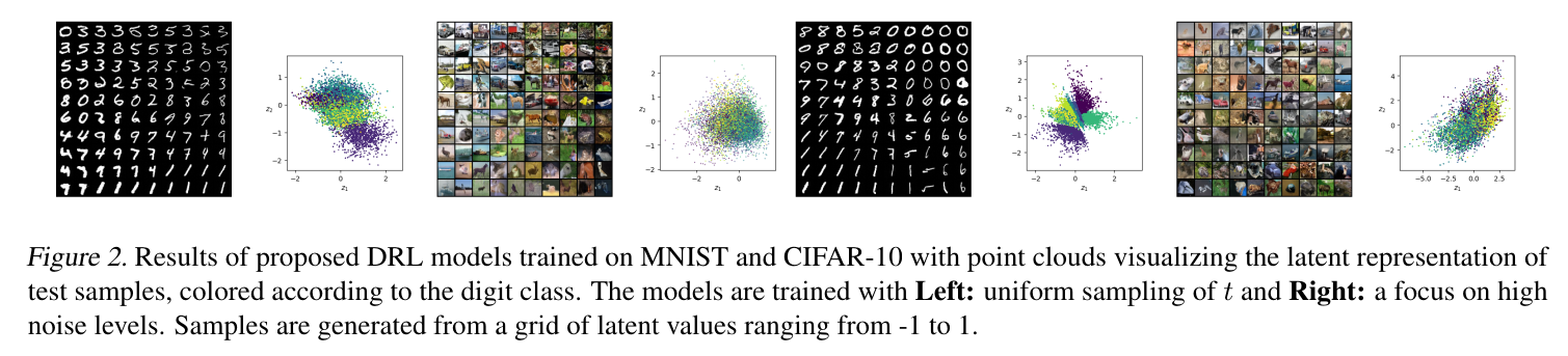
Paper 2: Diffusion and Representation Learning

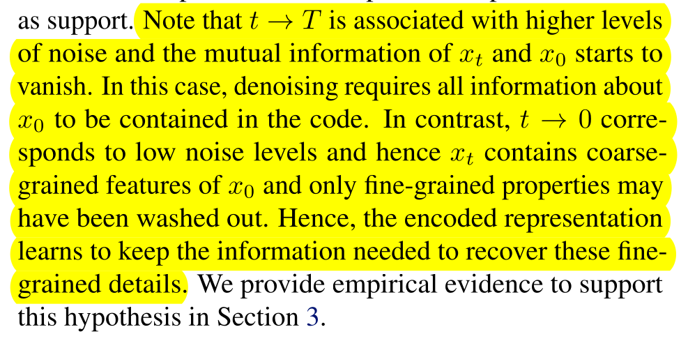
I have been thinking about images during diffusion process might contain different level of fidelity which we might want to exploit. This paper seems to realizes that idea. I really liked the proposed idea in the paper but the writing, particularly on mathematical derivations are quite clumsy and hard to follow.

Motivation

Representation learning uses 2 main approaches: contrastive learning and Non-contrastive learning (beta-VAE, denoising AE). While contrastive learning dominant the field, it requires additional supervising signals. So this works propose a way to learn some representation in a completely unsupervised way using diffusion model.

Why diffusion?

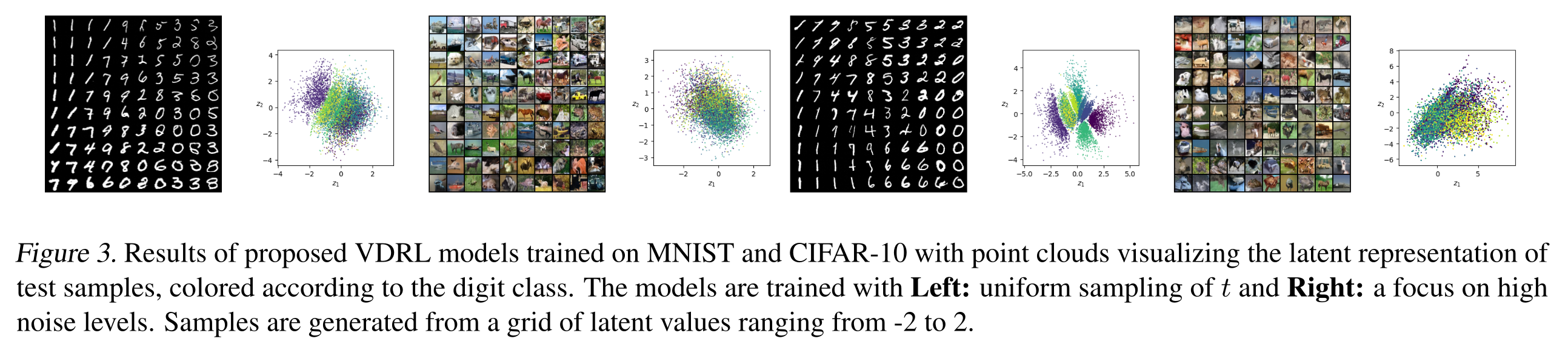
Proposed idea

Recall the score matching objective for unconditional diffusion model:

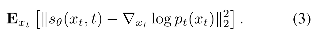
which can be learned approximately via a practical objective

Now suppose we want to train a conditional diffusion model given labeled data $(\textbf{x}, y(\textbf{x}))$, the objective would change to

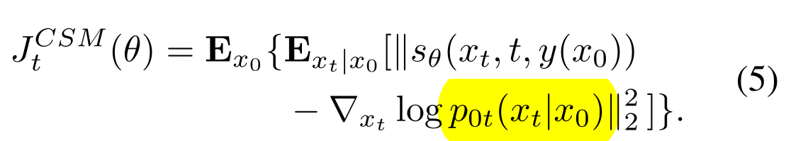
From that perspective, they propose to substitute $y(\textbf{x} _0)$ with an trainable encoder $\textbf{E} _{\boldsymbol \phi}(\textbf{x}_0)$.

Reasoning

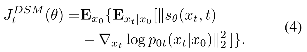
The objective of denoising score matching is equivalent to the probabilistic view (under certain parameterization). Particularly, the equation in (4) is equivalent to (if the forward step is to add a Gaussian noise)

We can see that minimizing the obj above, equivalently the obj in (4) is meant to make $\textbf{s} _{\boldsymbol \theta}(\widetilde{\textbf{x}}, \sigma)$ learn the direction toward $\textbf{x}$ or ($\textbf{x} _0$ in (4)) starting from $\widetilde{\textbf{x}}$(or $\textbf{x} _t$ in (4)). If $\textbf{s} _{\boldsymbol \theta}$ has access to additional information of $\textbf{x} _0$, via $\textbf{E} _{\boldsymbol \phi}(\textbf{x} _0)$, then it is hypothesized that $\textbf{E} _{\boldsymbol \phi}(\textbf{x} _0)$ would be able learn that direction, and hence help recover $\textbf{x} _0$.

Also, a side point is that having $\textbf{E} _{\phi}$ to optimize allow to get to a lower objective value. So at least $\textbf{E} _{\phi}$ makes certain different (the model cannot ignore that input).

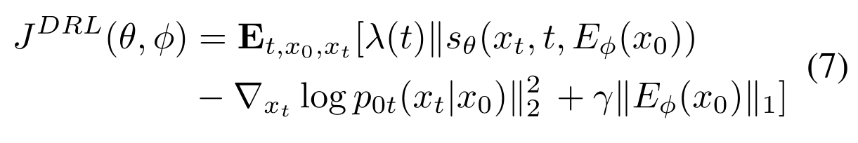
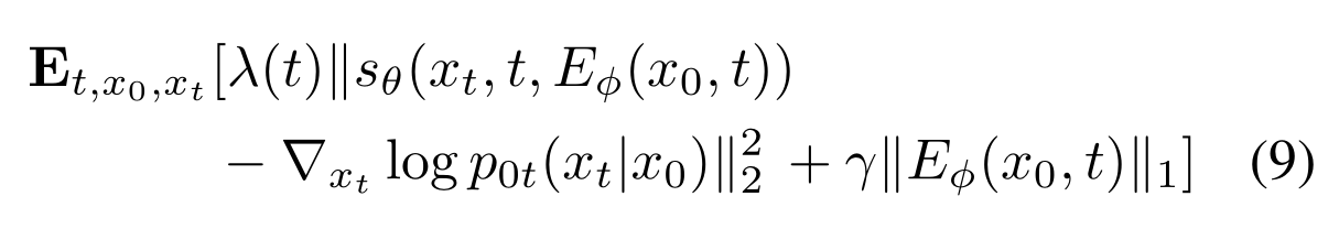
And lastly, the author proposed to include time step $t$ in the encoder’s parameters. Final objective function is

Performance

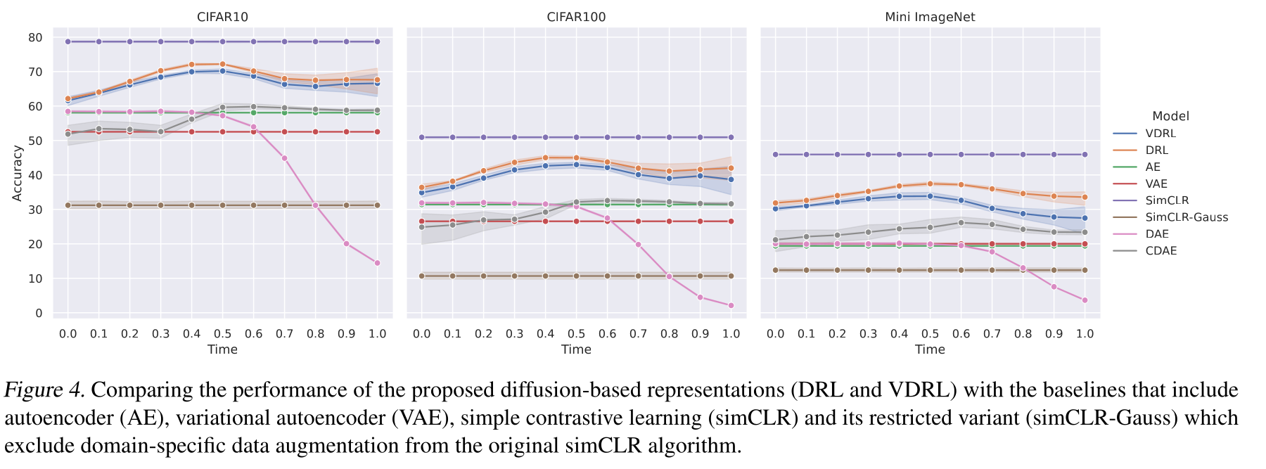
Some comments

• The proposal of using $\textbf{E}_{\boldsymbol \phi}$ seems quite heuristic. Don’t know if there a theory/principle way to back it up.
• Performance/experiment is not very surprising or convincing

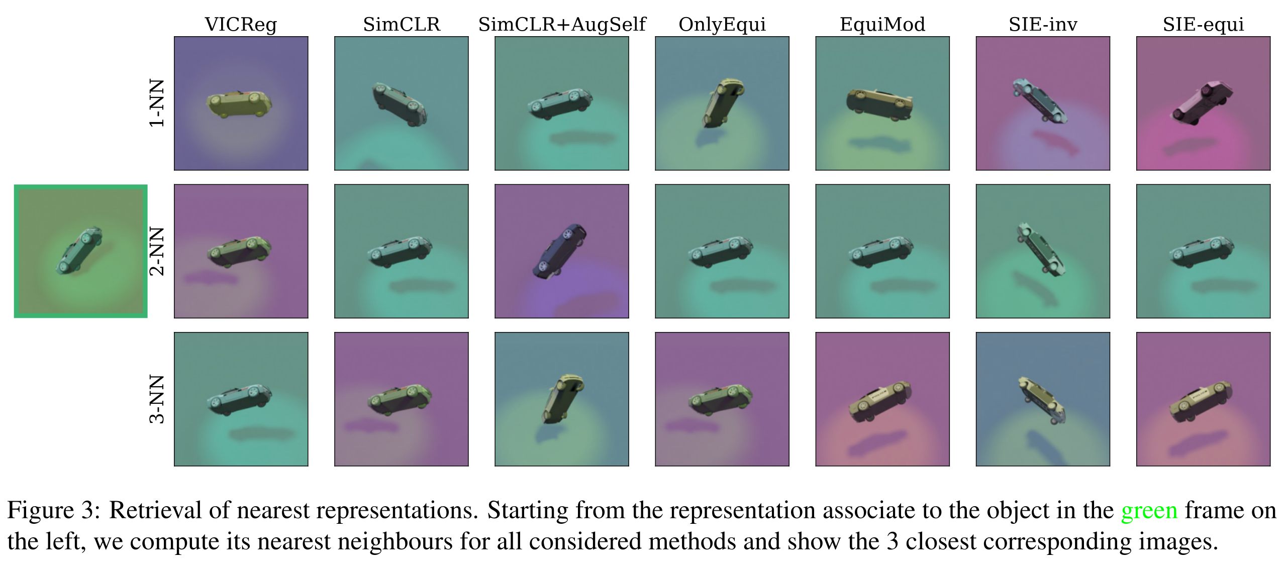
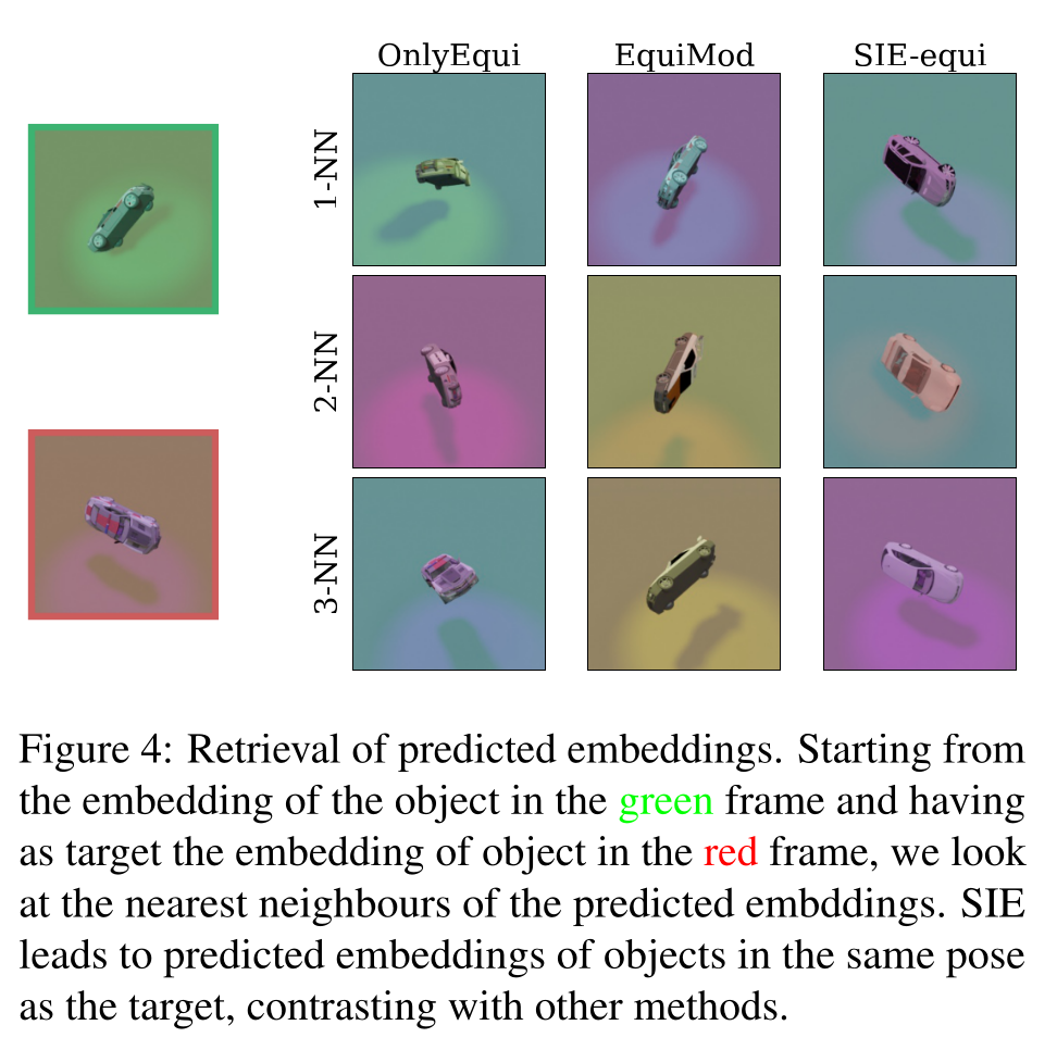
Paper 3: Equivariant in Representation Learning

Motivation

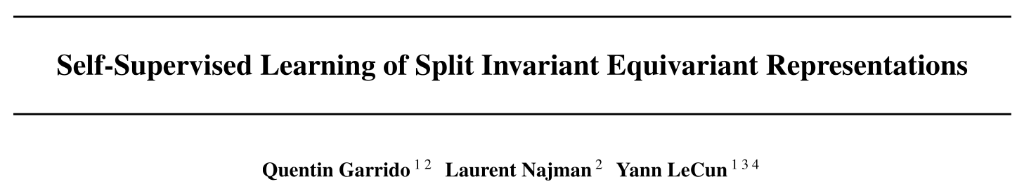
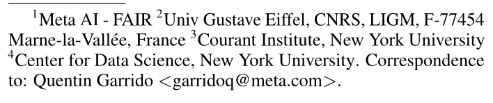
• What is equivariant?

What is a good representation? It should be low dimentional, invariant to unintersting transformation. Now people also propose that the latent should also contain information about transformation in a certain seperated elements.

Lots of papers on presentation learning is actually about how to distangled latent factors. And while it sounds intuitive, concrete defintion of distanglements are not completely agreed to each other. Among these, the work of [higgins2018towards] in which they soly proposed a very abstract but rigorous definition attracts quite a number of followers. And this paper is not an exception.

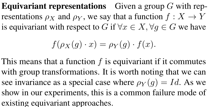
In words (in my understanding), equivariant requires that the latent vector contains all information about the transformation performed on the sample space so that there exists a transformation on the latten space to produce the same latent vector.

For reference, invariant is a special case of equivariant.

• Why do we care about equivariant?

It seems that learning latent vector to be invariant is quite intuitive and should be enough. However, for certain task, some augmentation transformation might accidentally destroy useful information. For instance, flower classification might want to use color as a feature, but color distoration augmentation might corrupt that information.

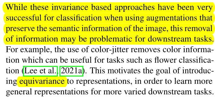
That is the only paragraph to motivate to learn equivariant in the paper. There may be more reason to acquire equivariant in the literature. For now, let’s take it for granted that learn an equivariant latent is a good thing to do. Let’s see how do they do it!

The problem setting and the goal

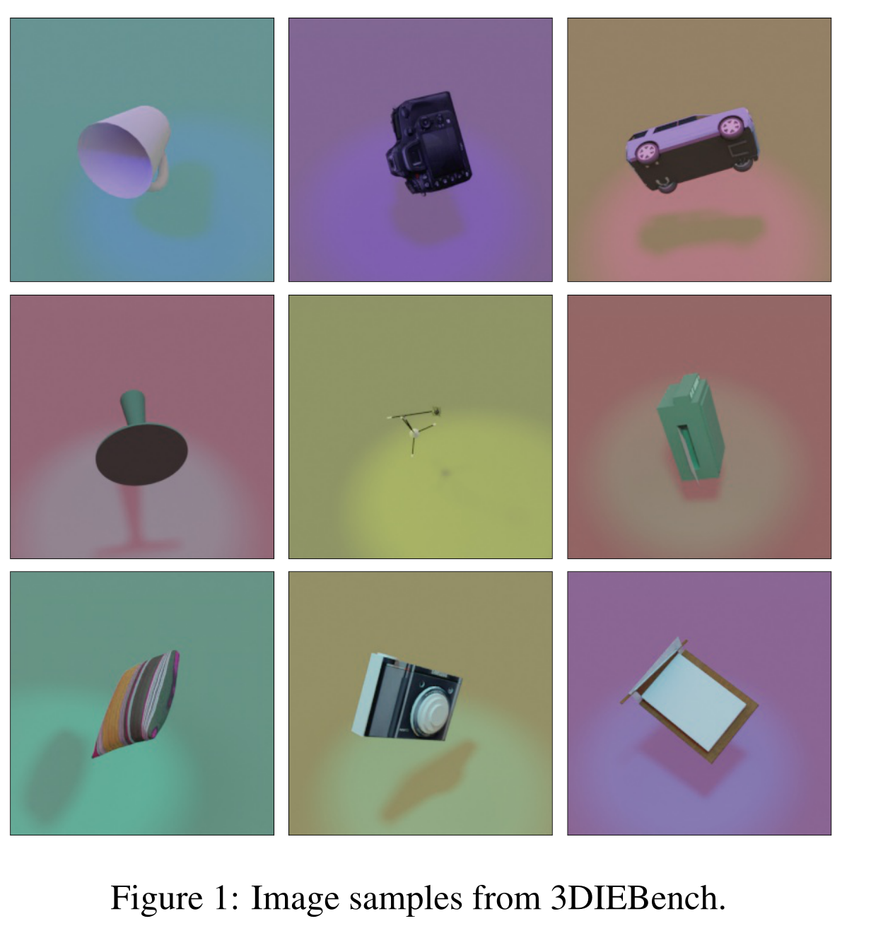
They first propose a 3D dataset (lets skip the part why do they need to do that, maybe current datasets aren’t good enough to show what they what to show). Each sample in this dataset contains:

• The image which is a 2D render of a 3D object.
• The class that the 3D object belongs to.
• The configuration that used to render 3D object to 2D images, including $x$-rotation angle, $y$-roration angle, $z$-rotation angle, light conditions, and colors.

Some image samples:

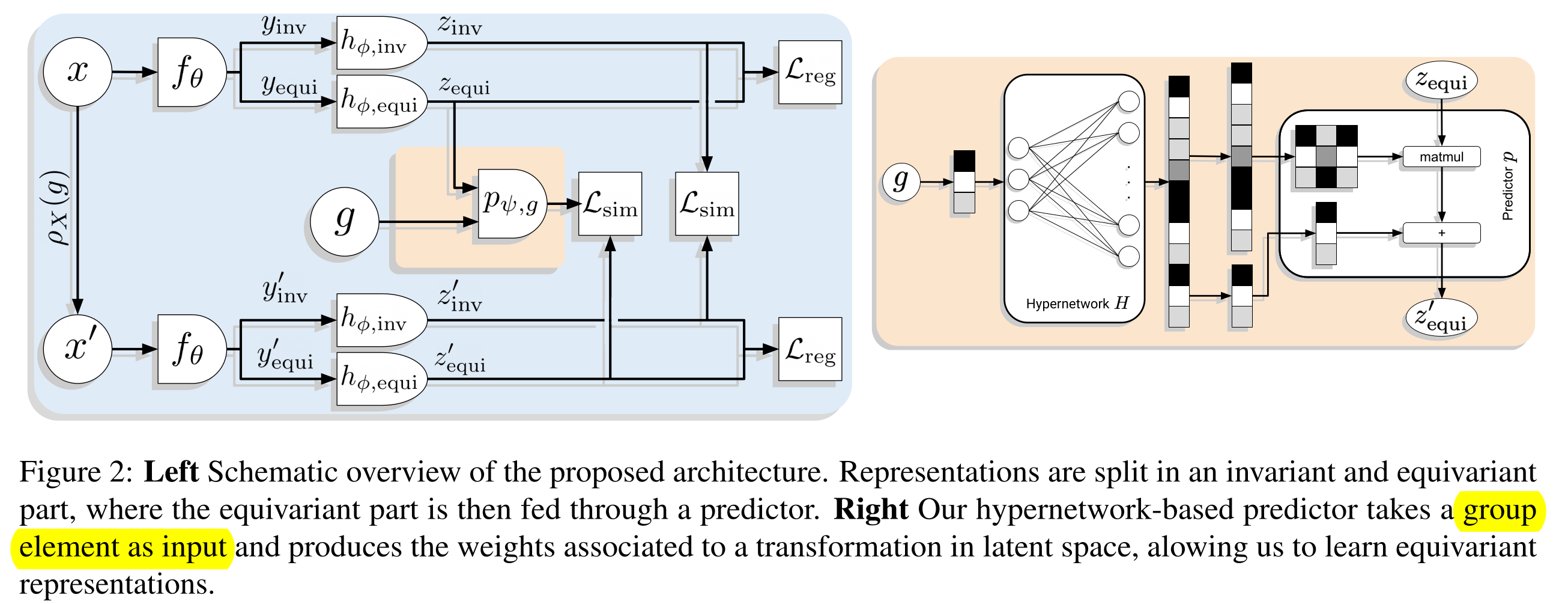
Task: Given sample $\textbf{x}$ as the 2D image rendering from a 3D object undergone a rotation transformation with known configurations (such as rotation angles), we want to learn 2 mappings:

• An encoder to map $\textbf{x}$ to its representation $\textbf{z}$,
• A mapping that map $\textbf{z}$ to $\textbf{z} _{ori}$ which is the latent of the before-transformed data point $\textbf{x}$. In their framework, these 2 mappings are $f$ and $\rho _{Y}$.

Proposal

Result

Paper 4: Another representation learning

Motivation

Rotation and translate transformation are meaningless in term of identifying meaningful object, hence the ideal representation should be invariant to those transformation. Existing methods are not always do that task well on complex datasets such as semiconductor wafer maps or plankton microscope images.

Also, my guess is that people don’t really augment data with very large angle for rotation like they do in this work ($[0, 2\pi]$).

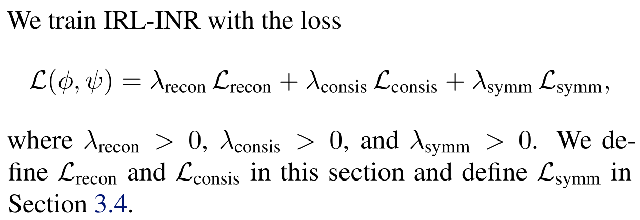
Task We want to learn a latent representation such that it is invariant to rotation and translation.

Proposal

Using implicit neural representation: viewing an 2D image as a function $\textbf{f}(x, y): \mathbb{R} \times \mathbb{R} \to \mathbb{R}^{c}$, where $c$ is the number of channels. This is the only interesting part of this paper (to me). The INR was proposed since 2007 and then getting popular 2-3 years recently.

With that in mind, we now can model the generative process involving translation and rotation. It is worth noting (surprising to me) that we have no idea how to model rotation transformation on sample space.

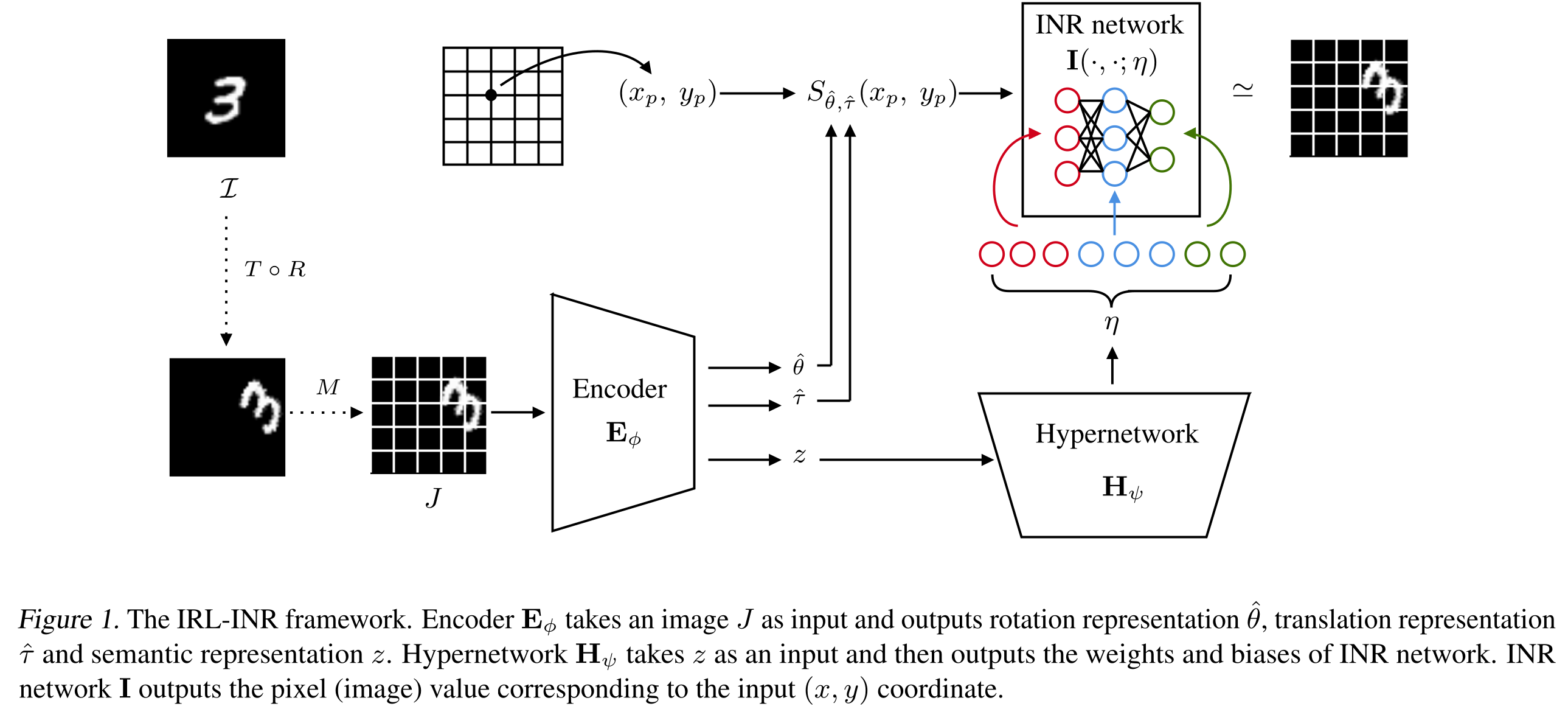
With this mechanism, rotation and translation parameters are just 2 extra parameters beside the latent vector. We will learn all these parameters using several (intuitively derived) losses.

• And the symm loss, cover later …

Result

Visually speaking, the result looks quite interesting. Note image is the only input.

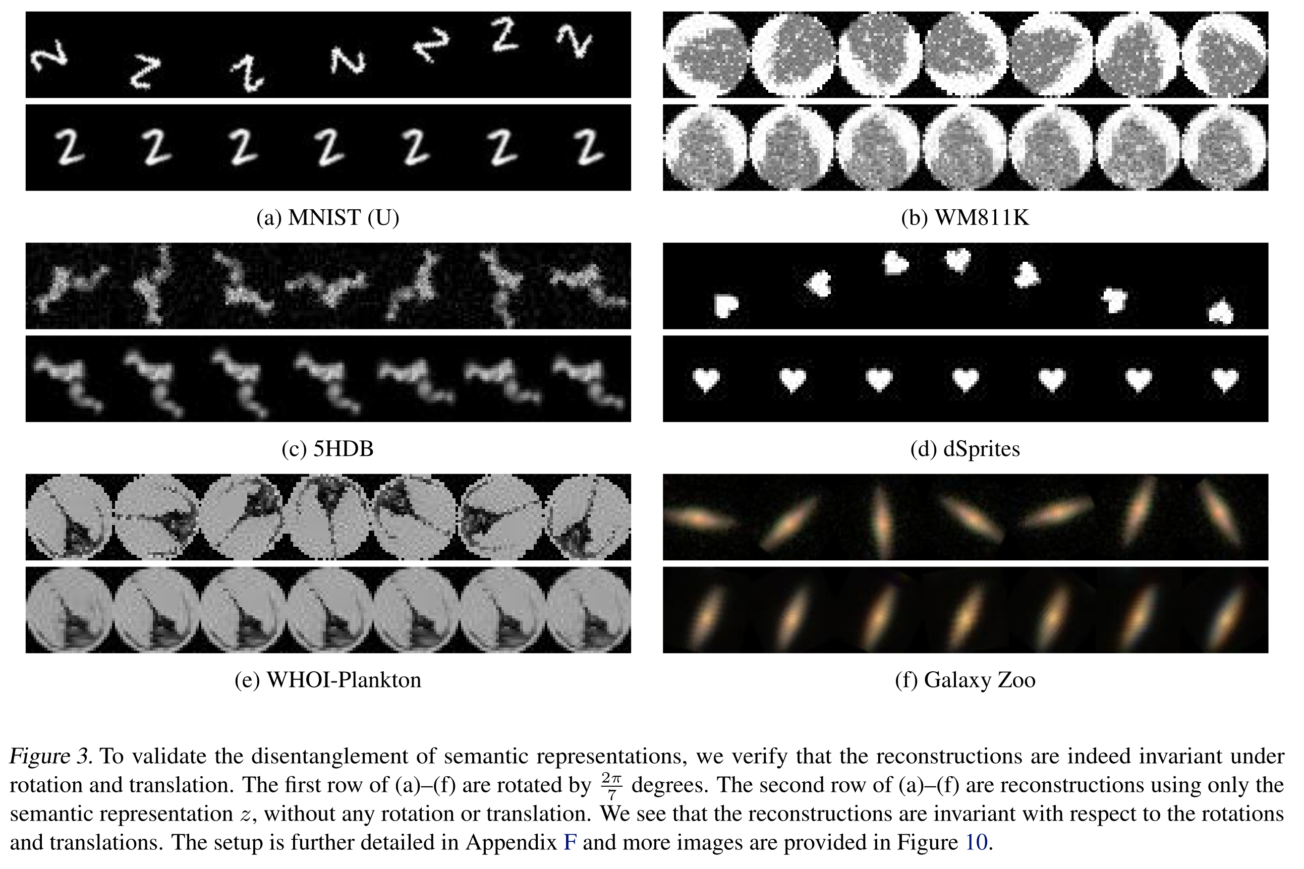
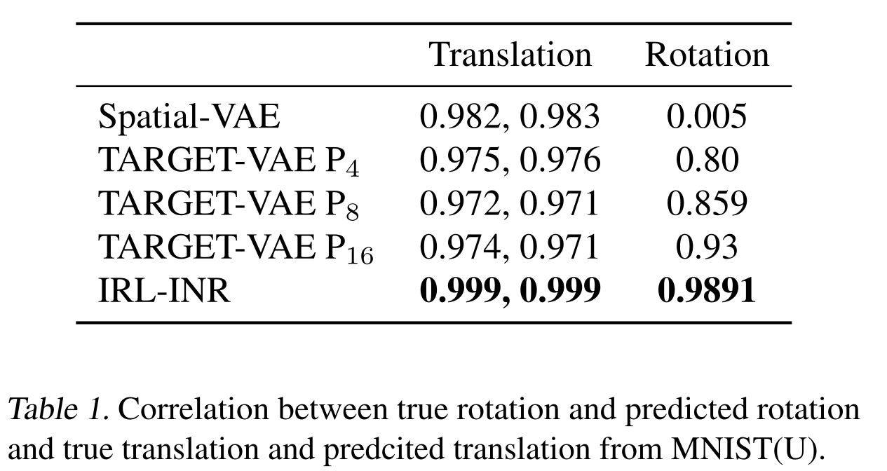Note that all baselines use INR.

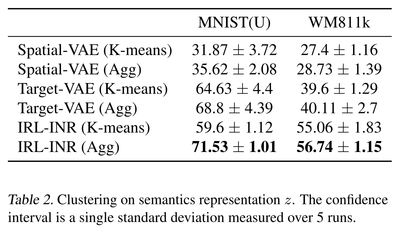
• How about disentangle?

Paper 5: Yet another representation learning paper

Motivation

Latent representation should store information in a hierchachy like the way human think.

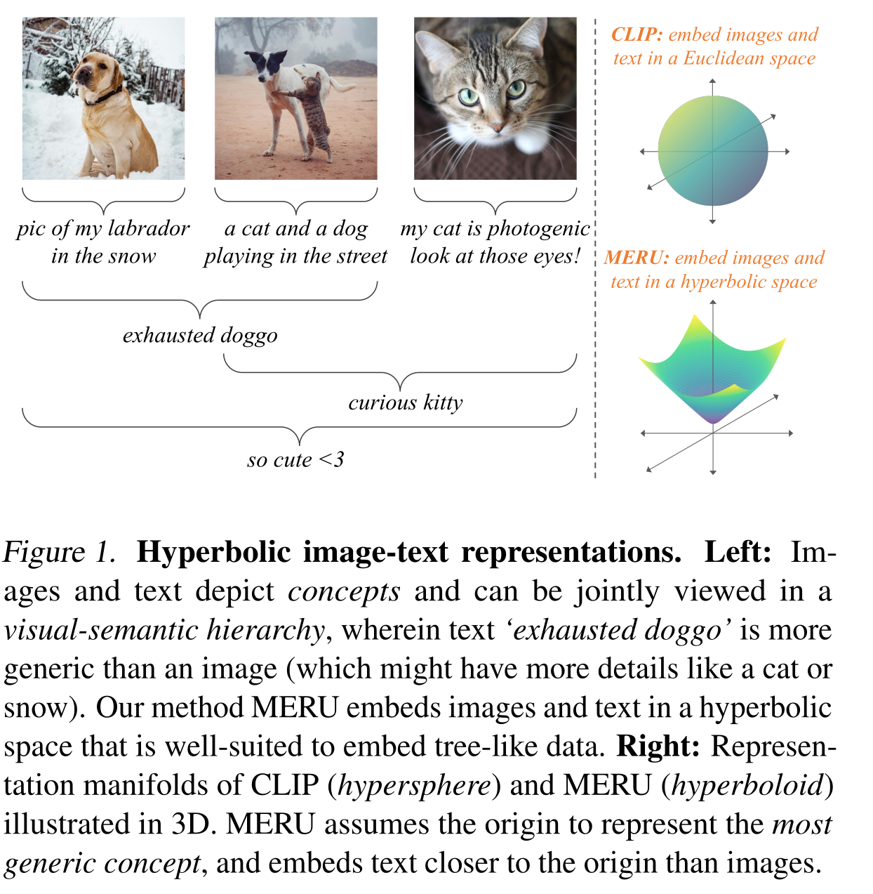
Proposal

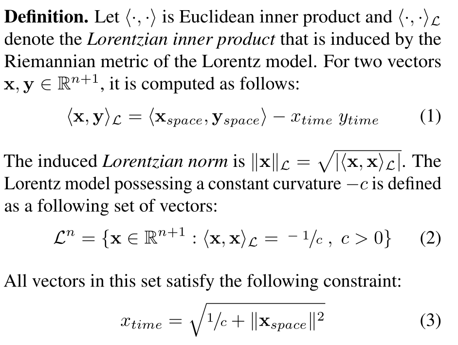
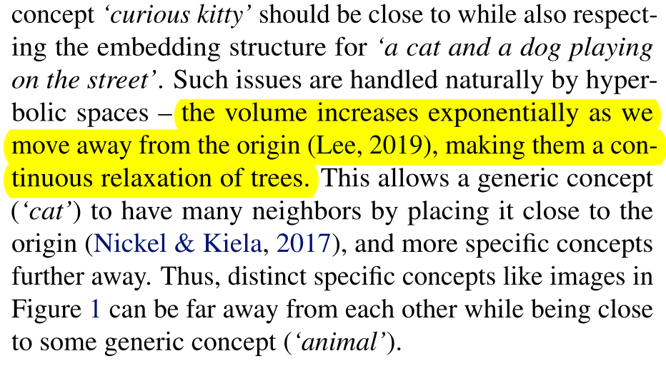
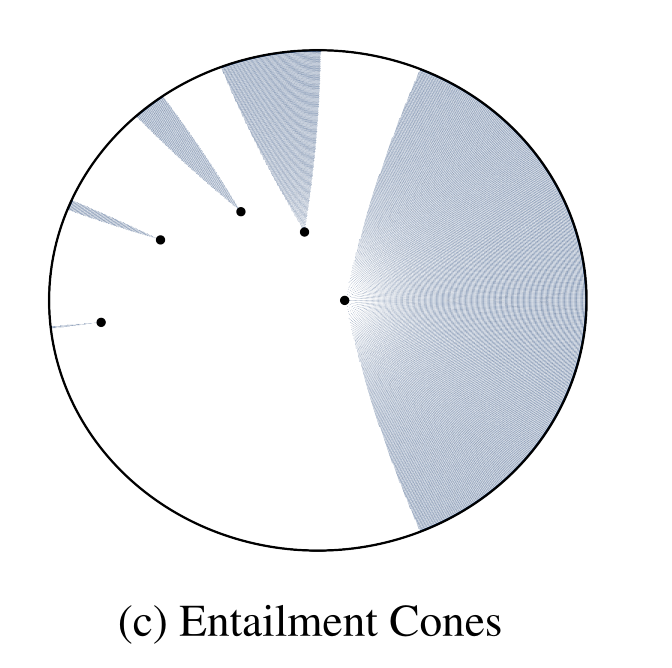
Break up with the Euclidean space, move to the hyperbolic space. Some definitions, but I wont cover all in details.

The important feature of this space is:

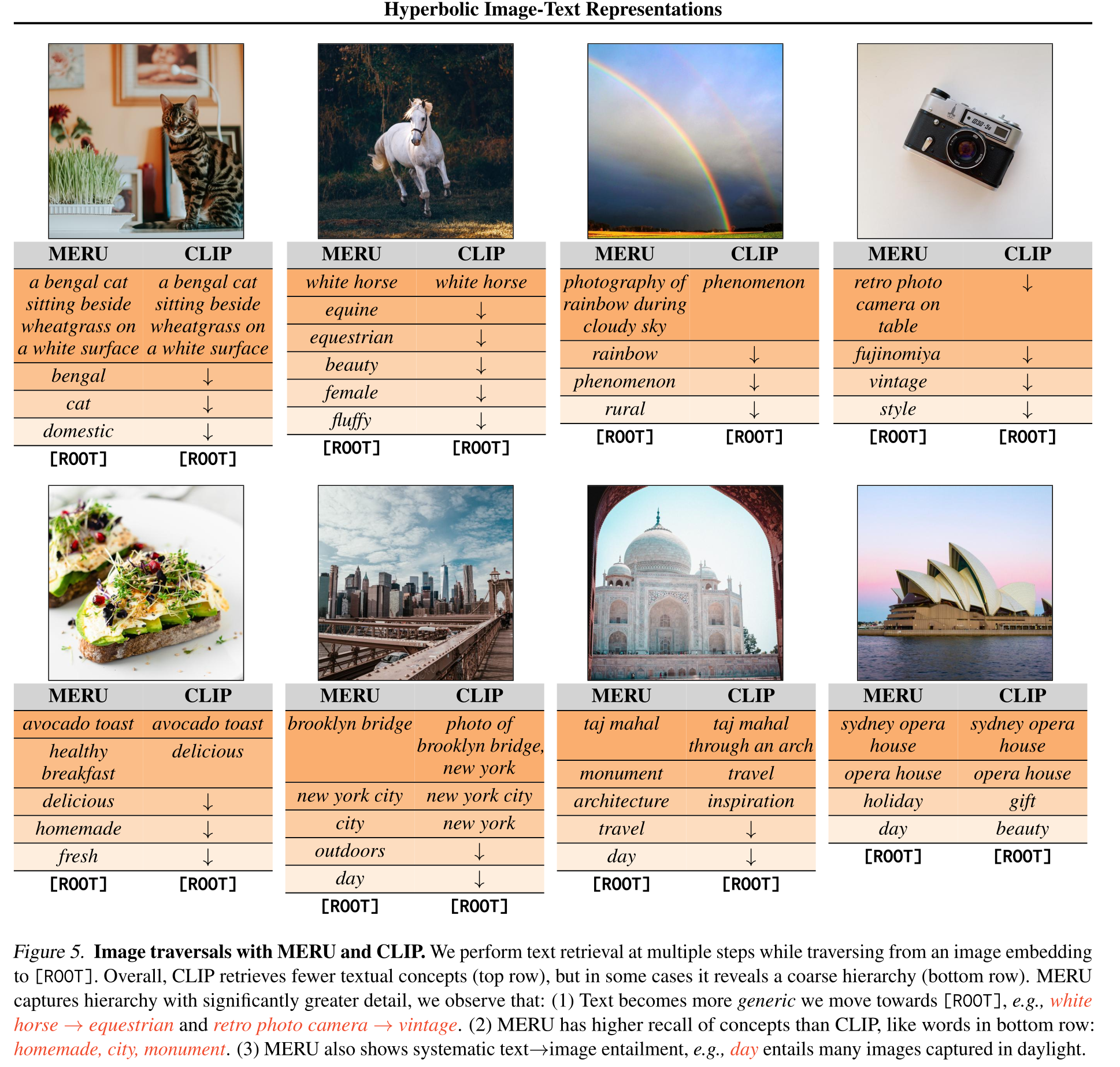
• The losses: Contrastive loss + Entailment loss

Contrastive loss is realized like in the CLIP paper. Given pair of text, image, model tries to predict which matches which.

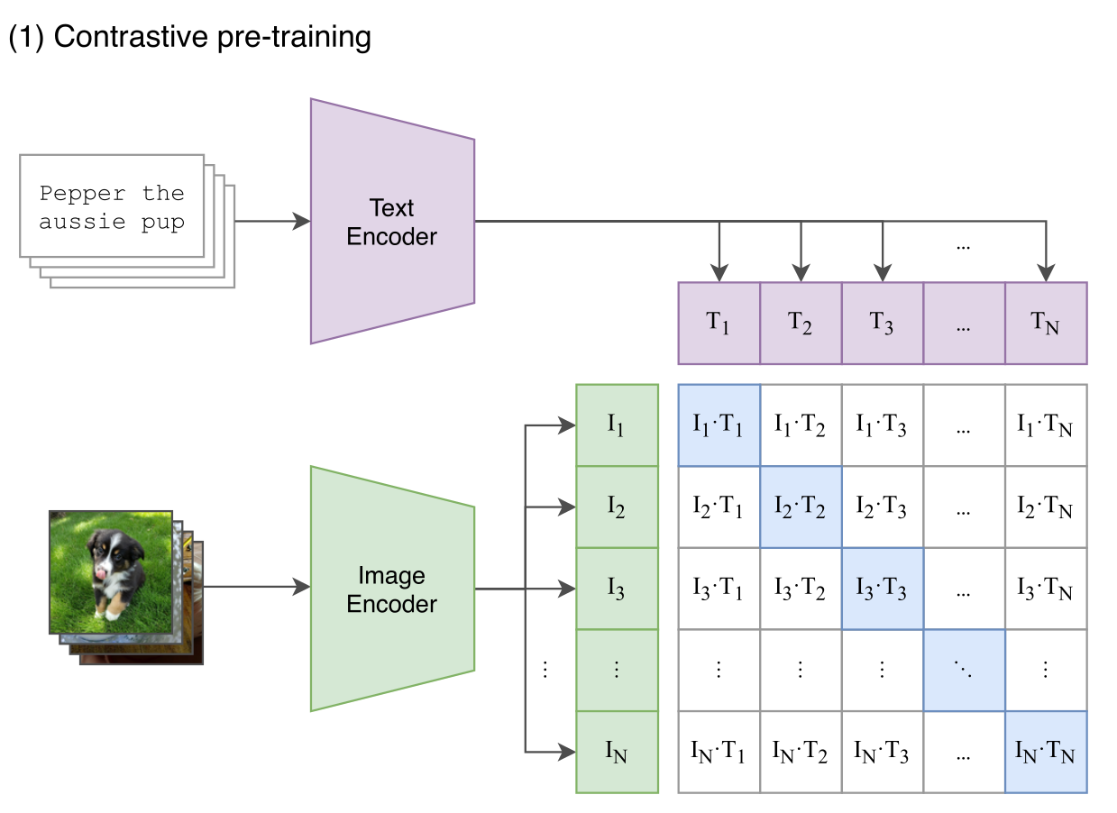(from CLIP paper)

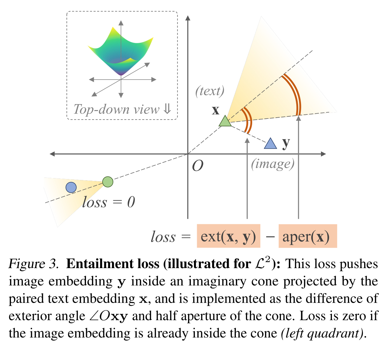
The entailment loss is used to model the relationship ($\textbf{u}$, “is a”, $\textbf{v}$)

Result

Look quite interesting!!!